Analyzing 3 Million Taxi Trips in the Browser: A Parquet + CSV Workbench Test
The question
Can you answer a real question about a few million rows of data in a browser tab, without uploading the file anywhere and without installing anything?
To check, we picked one concrete task and did it end to end with the site's existing Parquet Viewer and DuckDB Playground:
Using the January 2024 NYC yellow-taxi trip records, how does tipping on credit-card trips differ by pickup borough?
That task needs a large Parquet file, a small CSV lookup table, a join between them, some data-quality filters, and an aggregate. We recorded file sizes, timings, memory and network traffic, compared the answer with native DuckDB, and then pushed the tools until they slowed down.
This post is about the workflow. For why Parquet files are so much smaller than JSON or CSV, see Storing 2M analytics events: from JSON to Parquet and DuckDB. For profiling a CSV or JSON file's columns before you analyze it, see Profile CSV and JSON files without uploading them.
The data
Both files are public and come from the NYC Taxi & Limousine Commission (TLC) trip record data:
| File | Size | Rows | Columns | SHA-256 (first 8) |
|---|---|---|---|---|
yellow_tripdata_2024-01.parquet | 47.6 MB (49,961,641 bytes) | 2,964,624 | 19 | c4d59da7 |
taxi_zone_lookup.csv | 12 KB (12,331 bytes) | 265 | 4 | 1a99e105 |
The trip file has one row per trip, with pickup and drop-off times, a pickup zone ID (PULocationID), payment type, fare, tip and other charges. The lookup CSV maps each zone ID to a borough and zone name.
One detail decides the shape of the analysis. The TLC data dictionary says tip_amount is filled in automatically for credit-card tips and cash tips are not included. A cash trip with tip_amount = 0 tells you nothing about whether the passenger tipped. So the analysis only looks at credit-card trips (payment_type = 1).
Environment
- Machine: Linux laptop, AMD Ryzen 7 5825U (8 cores, 16 threads), about 27 GB RAM, Ubuntu 26.04.
- Browser: Chromium 145.0.7632.6, headless, 1440×900 viewport, driven by a Playwright script. The script used the pages the same way a person would: it chose files with the pages' own file inputs, typed SQL into the editor and pressed Run.
- Site: the timings below are from the production site, www.devtoolsdaily.com, 3 runs, each with a fresh browser profile (cold cache). Analytics and Firebase requests were blocked so they wouldn't add noise. We also ran the same workflow 3 times against a local development build; those results were identical and the timings similar. The screenshots are from the development build.
- Engine: both tools run DuckDB-Wasm 1.29.0, which is DuckDB v1.1.1 compiled to WebAssembly.
- Reference: native DuckDB 2.0.0 (the Python package) on the same machine, used only to check the browser's answers.
The workflow
Step 1: Check the file in the Parquet Viewer
Open the Parquet Viewer and choose yellow_tripdata_2024-01.parquet. The header shows the size, row count and column count. The Schema tab lists the 19 columns with their types, so you can confirm the column names before writing SQL: tpep_pickup_datetime, PULocationID, payment_type, fare_amount, tip_amount and so on.
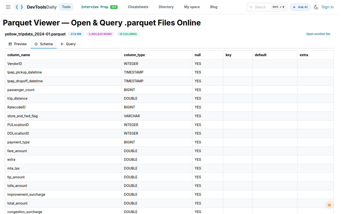
Over the three production runs, the file was open with its preview visible 2.4 s after it was chosen (2,365–2,451 ms). That includes downloading the DuckDB engine on first use.
The viewer is good for a first look. It reads one file, though, and our task needs a join with a second file, so the next step moves to the playground.
Step 2: Add both files to the DuckDB Playground
Open the DuckDB Playground and add both files to it. Each file shows up under Data sources in the Explorer and can be queried by its file name, for example FROM 'yellow_tripdata_2024-01.parquet'.
The Playground's Data sources list only shows files added on the Playground page, so add the file again even if you just opened it in the Viewer.
Registering the 47.6 MB Parquet file took 1.2 s (1,138–1,297 ms); the 12 KB CSV took about 35 ms.
Step 3: Run data-quality checks
Before computing anything, count the rows that would distort the answer:
SELECT
  count(*) AS trips,
  count(*) FILTER (WHERE tpep_pickup_datetime < '2024-01-01' OR tpep_pickup_datetime >= '2024-02-01') AS outside_january,
  count(*) FILTER (WHERE tpep_dropoff_datetime < tpep_pickup_datetime) AS dropoff_before_pickup,
  count(*) FILTER (WHERE fare_amount <= 0) AS non_positive_fare,
  count(*) FILTER (WHERE payment_type = 1) AS credit_card,
  count(*) FILTER (WHERE payment_type = 2) AS cash
FROM 'yellow_tripdata_2024-01.parquet';
Open this query in the DuckDB Playground. The link carries only the SQL. Your data files never go into a link, so you have to add them yourself.
| trips | outside_january | dropoff_before_pickup | non_positive_fare | credit_card | cash |
|---|---|---|---|---|---|
| 2,964,624 | 18 | 56 | 38,341 | 2,319,046 | 439,191 |
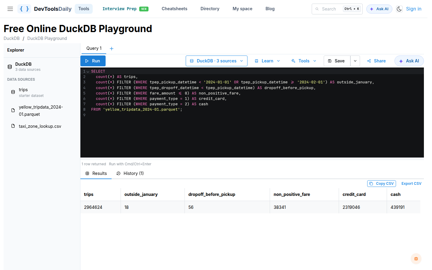
The query scanned the whole file in about 0.9 s (872–966 ms). The problem rows are few, but they exist, so the main query filters them out.
Step 4: Answer the question
Join the trips to the zone lookup, keep clean credit-card trips, and aggregate by pickup borough:
SELECT
  z.Borough AS pickup_borough,
  count(*) AS card_trips,
  round(100.0 * count(*) FILTER (WHERE t.tip_amount = 0) / count(*), 1) AS no_tip_pct,
  round(median(t.tip_amount / t.fare_amount) * 100, 1) AS median_tip_pct_of_fare,
  round(median(t.fare_amount), 2) AS median_fare
FROM 'yellow_tripdata_2024-01.parquet' AS t
JOIN 'taxi_zone_lookup.csv' AS z ON z.LocationID = t.PULocationID
WHERE t.payment_type = 1
  AND t.fare_amount > 0
  AND t.tip_amount >= 0
  AND t.tpep_pickup_datetime >= '2024-01-01'
  AND t.tpep_pickup_datetime < '2024-02-01'
  AND t.tpep_dropoff_datetime >= t.tpep_pickup_datetime
GROUP BY ALL
ORDER BY card_trips DESC;
Open this query in the DuckDB Playground
The filters left 2,318,840 trips, and every one matched a zone in the lookup.
| Pickup borough | Card trips | No tip | Median tip, % of fare | Median fare |
|---|---|---|---|---|
| Manhattan | 2,086,919 | 3.8% | 26.6% | $12.10 |
| Queens | 201,921 | 8.9% | 23.1% | $52.70 |
| Brooklyn | 15,788 | 68.9% | 0.0% | $26.50 |
| Unknown | 7,973 | 5.0% | 25.4% | $12.80 |
| Bronx | 5,000 | 95.9% | 0.0% | $34.50 |
| N/A | 966 | 35.0% | 8.3% | $90.00 |
| EWR | 251 | 23.9% | 17.2% | $108.00 |
| Staten Island | 22 | 36.4% | 10.3% | $83.45 |
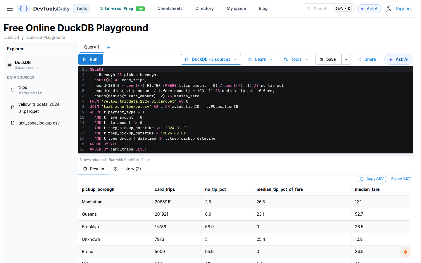
The join and aggregate took about 0.75 s (709–831 ms) on first run and about 0.6 s when run again.
What the result says, and what it doesn't:
- 90% of the card trips start in Manhattan. There, and in Queens (which includes JFK and LaGuardia), almost every card trip has a tip, with a median of about a quarter of the fare.
- Brooklyn and the Bronx look very different. 68.9% and 95.9% of their card trips have a recorded tip of zero. They are also small groups (15,788 and 5,000 trips). The trip records don't say why, so we don't guess.
- "Unknown" and "N/A" are rows in the TLC lookup, not join failures. Zone 264 has the borough "Unknown", and zone 265 ("Outside of NYC") has the borough "N/A". We kept them in the result rather than hiding them.
- EWR (Newark Airport) and Staten Island are tiny groups, at 251 and 22 trips. Their percentages swing a lot with a few trips.
Step 5: Export and cross-check
Export CSV under the result grid downloaded the 8-row result. We ran the same SQL in native DuckDB 2.0.0 against the same two files, and every value matched. The browser's CSV was byte-identical across all six runs (3 on production, 3 on the development build).
Two formatting differences from the native output are worth knowing about if you feed the export to another tool:
- Count columns (DuckDB
BIGINT) are exported as quoted strings, for example"2086919". - Whole numbers lose their decimal part, for example
0instead of0.0.
Neither changes a value, but a strict CSV reader may read the counts as text.
What stayed on the machine
During the production runs we logged every network request the page made:
- Engine code from public CDNs: DuckDB-Wasm 1.29.0 and Apache Arrow from
cdn.jsdelivr.net, plus DuckDB's Parquet extension fromextensions.duckdb.org. The largest part,duckdb-eh.wasm, is 6.2 MB compressed (35.7 MB uncompressed). The engine, worker and Parquet extension total about 6.9 MB compressed. This is a one-time download per cold cache. - Normal page traffic: the site's own pages and scripts, fonts, and on each page load a small
GETto the site's API (api.devtoolsdaily.com) for the sidebar sponsor spotlight. - No data: the largest request body the page tried to send was 130 bytes. Neither the 47.6 MB Parquet file nor the CSV was sent anywhere. Both tools read files with the browser's File API and hand the bytes to DuckDB in the same tab.
This trace covers this workflow with analytics and Firebase requests blocked. It shows that the files stayed local; it isn't a full account of what every part of the site sends.
If you work offline or behind a strict firewall, keep in mind that the engine itself has to come from those CDNs the first time.
Where it slowed down
The task itself was fast. To find the limits, we kept going.
A 10× bigger file still worked. We added the January 2024 high-volume for-hire vehicle file (fhvhv_tripdata_2024-01.parquet, 473 MB, 19,663,930 rows) to the playground on production:
- Registering it took 3.0 s.
count(*)returned 19,663,930 in 0.9 s.- A per-company count with a median fare took 1.7 s. The numbers matched native DuckDB: HV0003 had 14,432,755 trips with a median base fare of $18.13, and HV0005 had 5,231,175 trips at $17.50.
- The browser's peak memory was 1.6 GB (all Chromium processes combined).
Big result sets are the real limit. The playground draws every returned row as a table row, so the cost is in showing results, not in running the query. Here is this query on production, with different values of n:
SELECT * FROM 'yellow_tripdata_2024-01.parquet' LIMIT n;
| Rows returned | Time until the grid showed them | Peak browser memory |
|---|---|---|
| 1,000 | 1.5 s | 1.0 GB |
| 10,000 | 6.0 s | 2.1 GB |
| 30,000 | 15.5 s | 4.4 GB |
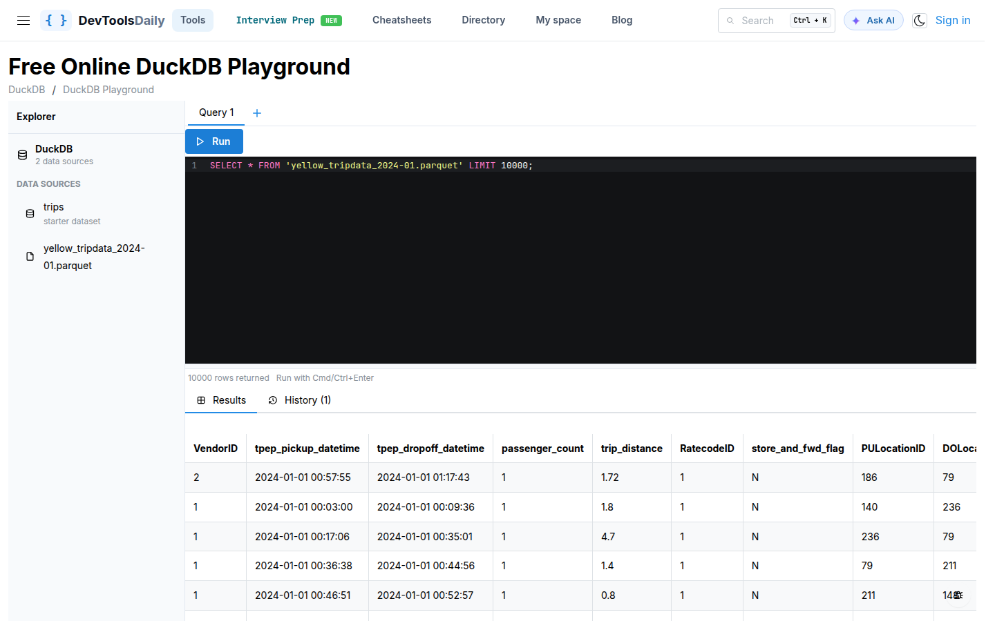
We stopped at 30,000 rows because memory was still growing quickly and the machine was shared with other work. On the local development build, which is slower, a 30,000-row result had not appeared after 150 s and a 100,000-row result had not appeared after 300 s.
The practical rule: aggregate or LIMIT inside SQL, and look at small results. A query that scans 3 million rows and returns 8 is fast. A query that returns 30,000 rows to the screen is not.
Other limits we ran into:
- Whole files are loaded into memory. Both tools read the entire file into the tab before querying it, so the file has to fit in the browser's memory along with everything else.
- Export is limited to the visible result. Export CSV and Copy CSV save the result that was returned to the grid. A DuckDB
COPY ... TO 'file.parquet'statement writes to DuckDB's in-browser file system, and neither tool has a button to download that file. So you can't use these pages to convert a large table to a new file. - Files don't carry between tools or links. You add files again when you switch tools, and a share link restores the SQL but not the files.
- The playground lists its sample table. The Explorer always shows a
tripsentry for the built-in starter dataset next to your files. It doesn't get in the way, but don't confuse it with your own data.
How this differs from the related posts
- Storing 2M analytics events measures storage: how big the same data is as JSON, CSV, SQLite and Parquet. This post doesn't compare formats. It measures doing an analysis in the browser on a file that is already Parquet.
- Profile CSV and JSON files without uploading them is about profiling columns, such as types, nulls and distinct values, before analysis. This post assumes you know what you want to ask and measures how far the browser tools take you.
Method and limitations
- One machine and one browser. The timings come from one laptop running headless Chromium. A phone, an older laptop or another browser will be different, and memory limits per tab vary by browser and device.
- Automated runs. A Playwright script did the clicks and typing. The timings measure the time from an action until the result appeared on the page, so they include rendering but not human think-time.
- Small number of runs. We ran the workflow 3 times on production and 3 times on a development build. We report the median and range from production, which is enough to show scale but not small differences.
- Engine versions differ. The browser tools run DuckDB v1.1.1 (through DuckDB-Wasm 1.29.0), and the cross-check used native DuckDB 2.0.0. The answers matched exactly for these queries, but other functions could behave differently between versions.
- One month, one dataset. The tipping results describe January 2024 yellow-taxi card trips only. They are not a claim about other months, cash trips or other trip types.
- Memory numbers are approximate. They are the combined resident memory of all Chromium processes, sampled while the step ran.
Try it
- Download
yellow_tripdata_2024-01.parquetandtaxi_zone_lookup.csvfrom the TLC. - Look at the trip file in the Parquet Viewer.
- Open the borough query in the DuckDB Playground, add both files, and press Run.
Related guides:
- How to inspect a Parquet file's schema
- How to query a CSV file with SQL
- Parquet file format explained
- Everything about DuckDB